import numpy as np
import anndata
import scanpy as sc
import mudata as md
from scipy import sparse
import pooch
import matplotlib.pyplot as plt
import pooch

Getting started with the anndata package

Suppose a colleague of yours did some single cell data analysis in Python and Scanpy, saving the results in an AnnData object and sending it to you in a *.h5ad file. This tutorial will walk you through that file and help you explore its structure and content — even if you are new to anndata, Scanpy or Python.

In this tutorial, we will refer to anndata as the package, and to its data structures as AnnData objects, respectively.

Exploring the AnnData object

We will use a preprocessed PBMC data set for our example. It is hosted on figshare and will be downloaded using the pooch package. The following line downloads the file scverse-getting-started-anndata-pbmc3k_processed.h5ad into ./data (ca. 100MB).

datapath = pooch.retrieve(
    url="https://figshare.com/ndownloader/files/40067737",
    known_hash="md5:b80deb0997f96b45d06f19c694e46243",
    path="./data",
    fname="scverse-getting-started-anndata-pbmc3k_processed.h5ad",
)

Now we can open it: Given a path to a *.h5ad file, read_h5ad will load the file into python and create our first AnnData object adata:

adata = anndata.read_h5ad(datapath)

(To load any *.h5adfile that already is on you machine, you would use adata = anndata.read_h5ad('path/to/file.h5ad'))

Let’s have a first look at the AnnData object:

adata

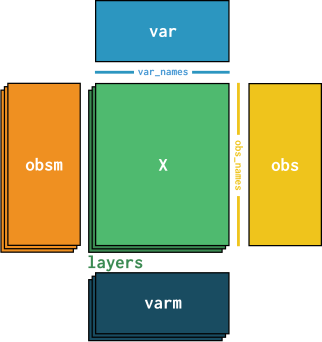
AnnData object with n_obs × n_vars = 2638 × 11505
    obs: 'n_genes', 'percent_mito', 'n_counts', 'louvain_cell_types'
    var: 'gene_names', 'n_cells', 'gene_ids'
    uns: 'louvain', 'louvain_colors', 'pca'
    obsm: 'X_pca', 'X_tsne', 'X_umap'
    layers: 'raw'
    obsp: 'distances_all'

This output tells us some general things about the data: its shape (2638 cells, 13714 genes) and which metadata fields and subfields it has. We will go through those one-by-one - let’s start with the most important one:

The active data matrix in adata.X

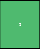
The adata.X slot holds the data matrix that we are actively using for analysis (e.g. for plotting gene expression values). That also means that most functions will use this data as input by default, unless explicitly told otherwise.

In this example, adata.X holds the matrix of normalized and log(1+x)-transformed mRNA counts. Its rows are cells (or observations), and its columns are genes (or variables).

adata.X

<2638x11505 sparse matrix of type '<class 'numpy.float32'>'
	with 2076576 stored elements in Compressed Sparse Row format>

We see that the data matrix is stored in the scipy sparse matrix format for compression. In brief, that means that we only store the non-zero expression values and their coordinates/indices in the data matrix explicitly, knowing that all other values are zeros. This saves a lot of RAM and makes processing faster, but also changes how we can interact with this object compared to a “normal” dense array. For an overview of the functions that you can apply directly on sparse arrays, check the scipy.sparse docs for the csr array.

Here are some examples to show how the sparse format works:

# look at the non-zero values in the data
print(adata.X.data)
# look at their indices / positions in the data matrix
print(adata.X.indices)
# compute the fraction of non-zero entries
print(adata.X.nnz / np.product(adata.X.shape))

[0.6496621 0.6496621 1.0402015 ... 0.7506172 0.7506172 1.4713064]
[   19    52    58 ... 11498 11501 11504]
0.068420527186156

Alternative versions of the active data in layers

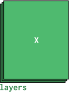
The data representation that we want to use mostly for plotting and processing lives in adata.X, e.g. the normalized counts. In addition to that, we often want to keep additional versions of our data around, e.g. the raw counts. These versions must have the exact same shape as adata.X and can be found in layers. Technically, layers is a Python dictionary and stores each layer under a separate key.

adata.layers

Layers with keys: raw

Our data only has a single additional layer, the raw counts, accessible via the layer key 'raw':

adata.layers["raw"]

<2638x11505 sparse matrix of type '<class 'numpy.int64'>'
	with 2076576 stored elements in Compressed Sparse Row format>

Its also a sparse matrix with the same shape as the active data in adata.X, but with integer values:

adata.layers["raw"].data

array([1, 1, 2, ..., 1, 1, 3])

Now let’s add a new layer, for example “counts per million”-normalized counts. We can compute it from the raw layer and store it in layers with a new name:

# copy raw counts to new layer
adata.layers["counts_per_million"] = adata.layers["raw"].copy()
# normalize the new layer to counts-per-million
sc.pp.normalize_total(adata, target_sum=10**6, layer="counts_per_million")
print(adata.layers)

Layers with keys: raw, counts_per_million

Also note that we had to explicitly tell the normalization function from Scanpy to use the new counts_per_million layer as input and output! Many functions in the scverse ecosystem support this through using the layer argument - for example the following plotting function from scanpy:

fig, (ax1, ax2) = plt.subplots(1, 2, figsize=(10, 2.5))
genes_of_interest = ["CD8A", "CD4", "KLRB1"]
sc.pl.matrixplot(
    adata,
    groupby="louvain_cell_types",
    var_names=genes_of_interest,
    layer="counts_per_million",  ## set which layer to plot
    ax=ax1,
    show=False,
)
ax1.set_title("CPM normalization")

sc.pl.matrixplot(
    adata,
    groupby="louvain_cell_types",
    var_names=genes_of_interest,
    layer="raw",  ## set which layer to plot
    ax=ax2,
    show=False,
)
ax2.set_title("raw counts")
plt.tight_layout()

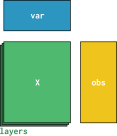
Simple annotations for cells and genes in obs and var

We usually want to store annotations for each cell and gene in adata.X. For cells, this can be the cluster assignments, batch IDs or a quality metric; for genes, it might be the gene name, ensembl ID or some measure of variance.

In AnnData objects, this information lives in adata.obs for cell annotations - each of its rows correspond to a row / cell in adata.X. Similarly, var holds the gene annotations.

adata.obs

	n_genes	percent_mito	n_counts	louvain_cell_types
cell_barcode
AAACATACAACCAC-1	781	0.030178	2419.0	CD4 T cells
AAACATTGAGCTAC-1	1352	0.037936	4903.0	B cells
AAACATTGATCAGC-1	1131	0.008897	3147.0	CD4 T cells
AAACCGTGCTTCCG-1	960	0.017431	2639.0	CD14+ Monocytes
AAACCGTGTATGCG-1	522	0.012245	980.0	NK cells
...	...	...	...	...
TTTCGAACTCTCAT-1	1155	0.021104	3459.0	CD14+ Monocytes
TTTCTACTGAGGCA-1	1227	0.009294	3443.0	B cells
TTTCTACTTCCTCG-1	622	0.021971	1684.0	B cells
TTTGCATGAGAGGC-1	454	0.020548	1022.0	B cells
TTTGCATGCCTCAC-1	724	0.008065	1984.0	CD4 T cells

2638 rows × 4 columns

This table is a Pandas Data Frame. We can see from its columns that we currently have four cell annotations:

• the number of genes per cell

• fraction of counts from mitochondrial genes in each cell (a quality metric)

• total counts per cell

• cell type assignment of a louvain clustering

All of these annotations are one-dimensional - they contain a single number or string per cell. Also, each cell is uniquely identified by the index of the table - in this case, the cell barcoding sequence (more about indexing in the next section).

To get a list of all cell annotations in the obs columns, you can use

adata.obs_keys()

['n_genes', 'percent_mito', 'n_counts', 'louvain_cell_types']

To access a specific column of the obs data frame, we can simply use its column name:

adata.obs["louvain_cell_types"]

cell_barcode
AAACATACAACCAC-1        CD4 T cells
AAACATTGAGCTAC-1            B cells
AAACATTGATCAGC-1        CD4 T cells
AAACCGTGCTTCCG-1    CD14+ Monocytes
AAACCGTGTATGCG-1           NK cells
                         ...       
TTTCGAACTCTCAT-1    CD14+ Monocytes
TTTCTACTGAGGCA-1            B cells
TTTCTACTTCCTCG-1            B cells
TTTGCATGAGAGGC-1            B cells
TTTGCATGCCTCAC-1        CD4 T cells
Name: louvain_cell_types, Length: 2638, dtype: category
Categories (8, object): ['CD4 T cells', 'CD14+ Monocytes', 'B cells', 'CD8 T cells', 'NK cells', 'FCGR3A+ Monocytes', 'Dendritic cells', 'Megakaryocytes']

Now, we can directly interact with these annotations, e.g. count the numbers of B cells in the data:

print(sum(adata.obs["louvain_cell_types"] == "B cells"))

342

To add a new cell annotations, we simply add a new column to the obs data frame.

For example, if we want to keep track of low-quality cells with a high mitochondrial gene count fraction, we can do the following to mark all cells above a certain threshold:

adata.obs["is_low_quality"] = adata.obs["percent_mito"] > 0.03
adata.obs  # to inspect the updated table

	n_genes	percent_mito	n_counts	louvain_cell_types	is_low_quality
cell_barcode
AAACATACAACCAC-1	781	0.030178	2419.0	CD4 T cells	True
AAACATTGAGCTAC-1	1352	0.037936	4903.0	B cells	True
AAACATTGATCAGC-1	1131	0.008897	3147.0	CD4 T cells	False
AAACCGTGCTTCCG-1	960	0.017431	2639.0	CD14+ Monocytes	False
AAACCGTGTATGCG-1	522	0.012245	980.0	NK cells	False
...	...	...	...	...	...
TTTCGAACTCTCAT-1	1155	0.021104	3459.0	CD14+ Monocytes	False
TTTCTACTGAGGCA-1	1227	0.009294	3443.0	B cells	False
TTTCTACTTCCTCG-1	622	0.021971	1684.0	B cells	False
TTTGCATGAGAGGC-1	454	0.020548	1022.0	B cells	False
TTTGCATGCCTCAC-1	724	0.008065	1984.0	CD4 T cells	False

2638 rows × 5 columns

The gene annotations in the var data frame work in the same way: Here, each row is a gene and in this example, the gene name is used as index. Additionally, the ensembl gene ID is available for each gene.

adata.var

	gene_names	n_cells	gene_ids
gene_names
LINC00115	LINC00115	18	ENSG00000225880
NOC2L	NOC2L	258	ENSG00000188976
KLHL17	KLHL17	9	ENSG00000187961
PLEKHN1	PLEKHN1	7	ENSG00000187583
HES4	HES4	145	ENSG00000188290
...	...	...	...
MT-ND4L	MT-ND4L	398	ENSG00000212907
MT-ND4	MT-ND4	2588	ENSG00000198886
MT-ND5	MT-ND5	1399	ENSG00000198786
MT-ND6	MT-ND6	249	ENSG00000198695
MT-CYB	MT-CYB	2517	ENSG00000198727

11505 rows × 3 columns

If you want to learn how to interact with the obs and var data frames in more advanced ways, you can have a look at these Pandas tutorials.

Index cells and genes with obs_names and var_names

One important aspect of AnnData objects is the shared indexing. Consider the case of cell annotations - no matter if we look at a cells raw counts, its cluster assignments or its k-nearest neighbors in the PCA space: we always want to be able to refer to the same cell with the same “name”. That is why all cell annotations share the same index, the obs_names. Similarly, we have var_names indexing our genes and their annotations. These annotations should be unique and many functions in the scverse ecosystem will raise warnings if this is not the case.

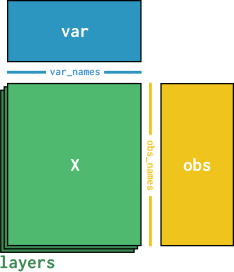
For the cells in our example data, the cell barcode from sequencing is used as index.

adata.obs_names

Index(['AAACATACAACCAC-1', 'AAACATTGAGCTAC-1', 'AAACATTGATCAGC-1',
       'AAACCGTGCTTCCG-1', 'AAACCGTGTATGCG-1', 'AAACGCACTGGTAC-1',
       'AAACGCTGACCAGT-1', 'AAACGCTGGTTCTT-1', 'AAACGCTGTAGCCA-1',
       'AAACGCTGTTTCTG-1',
       ...
       'TTTCAGTGTCACGA-1', 'TTTCAGTGTCTATC-1', 'TTTCAGTGTGCAGT-1',
       'TTTCCAGAGGTGAG-1', 'TTTCGAACACCTGA-1', 'TTTCGAACTCTCAT-1',
       'TTTCTACTGAGGCA-1', 'TTTCTACTTCCTCG-1', 'TTTGCATGAGAGGC-1',
       'TTTGCATGCCTCAC-1'],
      dtype='object', name='cell_barcode', length=2638)

Genes are indexed by gene name in this example:

adata.var_names

Index(['LINC00115', 'NOC2L', 'KLHL17', 'PLEKHN1', 'HES4', 'ISG15', 'AGRN',
       'C1orf159', 'TNFRSF18', 'TNFRSF4',
       ...
       'MT-CO2', 'MT-ATP8', 'MT-ATP6', 'MT-CO3', 'MT-ND3', 'MT-ND4L', 'MT-ND4',
       'MT-ND5', 'MT-ND6', 'MT-CYB'],
      dtype='object', name='gene_names', length=11505)

If needed, we can change the way cells or genes are indexed by using a different index array for obs_names or var_names. For that, we just need to set them to a new array of indices! For example, we can use the gene IDs instead of the gene name to index the genes:

adata.var_names = adata.var["gene_ids"]

As adata.var_names directly mirrors the index of adata.var, the index changes as expected:

adata.var

	gene_names	n_cells	gene_ids
gene_ids
ENSG00000225880	LINC00115	18	ENSG00000225880
ENSG00000188976	NOC2L	258	ENSG00000188976
ENSG00000187961	KLHL17	9	ENSG00000187961
ENSG00000187583	PLEKHN1	7	ENSG00000187583
ENSG00000188290	HES4	145	ENSG00000188290
...	...	...	...
ENSG00000212907	MT-ND4L	398	ENSG00000212907
ENSG00000198886	MT-ND4	2588	ENSG00000198886
ENSG00000198786	MT-ND5	1399	ENSG00000198786
ENSG00000198695	MT-ND6	249	ENSG00000198695
ENSG00000198727	MT-CYB	2517	ENSG00000198727

11505 rows × 3 columns

AnnData also automatically checks if the new index has the correct length - setting var_names with too few or too many indices will throw an error.

For now, let’s go back to the gene name index, as it is more interpretable:

adata.var_names = adata.var["gene_names"]
adata.var

	gene_names	n_cells	gene_ids
gene_names
LINC00115	LINC00115	18	ENSG00000225880
NOC2L	NOC2L	258	ENSG00000188976
KLHL17	KLHL17	9	ENSG00000187961
PLEKHN1	PLEKHN1	7	ENSG00000187583
HES4	HES4	145	ENSG00000188290
...	...	...	...
MT-ND4L	MT-ND4L	398	ENSG00000212907
MT-ND4	MT-ND4	2588	ENSG00000198886
MT-ND5	MT-ND5	1399	ENSG00000198786
MT-ND6	MT-ND6	249	ENSG00000198695
MT-CYB	MT-CYB	2517	ENSG00000198727

11505 rows × 3 columns

Subsetting AnnData objects

AnnData objects allow consistent subsetting of genes, cells or both. There are several options to subset:

• by name index (=var_names and/or obs_names) - in our example that would be lists of gene names ['LYZ','TUBB1','MALAT1'] or cell barcodes [AAACATACAACCAC-1', 'AAACATTGAGCTAC-1', 'AAACATTGATCAGC-1']

• by numerical index - e.g. :10 or 0:10 for the first 10 gene/cell, 5:10 for the sixth to the tenth, or [0,2,4] for the first, third and fifth

• by boolean index - e.g. our flag for low-quality cells adata.obs['is_low_quality'] or an index to all cells in the B cell cluster as in adata.obs['louvain']=='B cells'

All of these index operations can be combined, and will automatically subset the active data in adata.X, all layers, and all annotation fields to the selected subset. For example, if we want to get the first five cells in the data for three specific genes we are interested in, obs and var will be subsetted.

adata_small = adata[:5, ["LYZ", "FOS", "MALAT1"]]
adata_small.shape

(5, 3)

# active data (log-normalized counts) after subsetting
adata_small.X.A  # we use .A just for display reasons here:
# it turns the sparse data in X into a dense array that can be nicely printed

array([[0.6496621 , 2.4036813 , 3.8249342 ],
       [0.8553989 , 0.64266497, 4.174533  ],
       [0.878057  , 2.8014445 , 4.7918878 ],
       [3.0494576 , 1.6464083 , 2.3237872 ],
       [0.        , 0.        , 3.923651  ]], dtype=float32)

# raw data layer after subsetting
adata_small.layers["raw"].A

array([[  1,  11,  49],
       [  3,   2, 142],
       [  2,  22, 170],
       [ 24,   5,  11],
       [  0,   0,  22]])

# cell annotations after subsetting
adata_small.obs

	n_genes	percent_mito	n_counts	louvain_cell_types	is_low_quality
cell_barcode
AAACATACAACCAC-1	781	0.030178	2419.0	CD4 T cells	True
AAACATTGAGCTAC-1	1352	0.037936	4903.0	B cells	True
AAACATTGATCAGC-1	1131	0.008897	3147.0	CD4 T cells	False
AAACCGTGCTTCCG-1	960	0.017431	2639.0	CD14+ Monocytes	False
AAACCGTGTATGCG-1	522	0.012245	980.0	NK cells	False

# gene annotations after subsetting
adata_small.var

	gene_names	n_cells	gene_ids
gene_names
LYZ	LYZ	1631	ENSG00000090382
FOS	FOS	2473	ENSG00000170345
MALAT1	MALAT1	2699	ENSG00000251562

Lets also try some boolean indexing, where we keep the gene axis unchanged (using :), and keeping only the high quality cells (by inverting adata.obs['is_low_quality'] with the “NOT” operator ~)

adata_high_quality = adata[~adata.obs["is_low_quality"], :]

# obs data frame after subsettings shows that the low-quality cells are gone
adata_high_quality.obs

	n_genes	percent_mito	n_counts	louvain_cell_types	is_low_quality
cell_barcode
AAACATTGATCAGC-1	1131	0.008897	3147.0	CD4 T cells	False
AAACCGTGCTTCCG-1	960	0.017431	2639.0	CD14+ Monocytes	False
AAACCGTGTATGCG-1	522	0.012245	980.0	NK cells	False
AAACGCACTGGTAC-1	782	0.016644	2163.0	CD8 T cells	False
AAACGCTGTAGCCA-1	533	0.011765	1275.0	CD4 T cells	False
...	...	...	...	...	...
TTTCGAACTCTCAT-1	1155	0.021104	3459.0	CD14+ Monocytes	False
TTTCTACTGAGGCA-1	1227	0.009294	3443.0	B cells	False
TTTCTACTTCCTCG-1	622	0.021971	1684.0	B cells	False
TTTGCATGAGAGGC-1	454	0.020548	1022.0	B cells	False
TTTGCATGCCTCAC-1	724	0.008065	1984.0	CD4 T cells	False

2257 rows × 5 columns

Note:

Technically, subsetting AnnData objects returns a view of the AnnData you are subsetting from instead of making a copy. That avoids having the same data in memory twice. We describe the details of how views work in a separate section below.

Multidimensional annotations for cells and genes in obsm and varm

adata.uns.keys()

dict_keys(['louvain', 'louvain_colors', 'pca'])

Sometimes, the simple, one-dimensional annotations in obs and var are not enough to store the results of our analysis.

For example, if we embed our data with t-SNE or UMAP, we usually obtain a two-dimensional vector of embedding coordinates for each cell. For a PCA with, say, 50 components, we would even get a 50-dimensional vector per cell. To store these multidimensional representations of the cells, AnnData objects provide the obsm object.

For multidimensional information about genes, we have varm, which works similarly and could e.g. hold the PCA loadings for each gene.

Now, let’s have a look at our example adata.obsm:

adata.obsm

AxisArrays with keys: X_pca, X_tsne, X_umap

In our example, it contains representation of our cells after PCA, t-SNE and UMAP. Technically, these three representations are stored in a Python dictionary with separate keys.

We can look at the data shape for each of them:

for key in adata.obsm_keys():
    print(key, adata.obsm[key].shape, sep="\t")

X_pca	(2638, 50)
X_tsne	(2638, 2)
X_umap	(2638, 2)

The numbers of observations always has to be the same as in adata.X, but the number of dimensions can vary.

Also, let’s make a simple plot of the the first two PCs from PCA and the UMAP / t-SNE embeddings, and highlight the B cells:

plt.figure(figsize=(12, 4))

# PCA
plt.subplot(1, 3, 1)
plt.scatter(
    x=adata.obsm["X_pca"][:, 0],  # PCA dim 1
    y=adata.obsm["X_pca"][:, 1],  # PCA dim 2
    c=adata.obs["louvain_cell_types"] == "B cells",  # B cell flag
    s=3,
    linewidth=0,
    cmap="coolwarm",
)
plt.title("PCA")
plt.axis("off")
plt.gca().set_aspect("equal")

# t-SNE
plt.subplot(1, 3, 2)
plt.scatter(
    x=adata.obsm["X_tsne"][:, 0],  # t-SNE dim 1
    y=adata.obsm["X_tsne"][:, 1],  # t-SNE dim 2
    c=adata.obs["louvain_cell_types"] == "B cells",  # B cell flag
    s=3,
    linewidth=0,
    cmap="coolwarm",
)
plt.title("t-SNE")
plt.axis("off")
plt.gca().set_aspect("equal")

# UMAP
plt.subplot(1, 3, 3)
plt.scatter(
    x=adata.obsm["X_umap"][:, 0],  # UMAP dim 1
    y=adata.obsm["X_umap"][:, 1],  # UMAP dim 2
    c=adata.obs["louvain_cell_types"] == "B cells",  # B cell flag
    s=3,
    linewidth=0,
    cmap="coolwarm",
)
plt.title("UMAP")
plt.axis("off")
plt.gca().set_aspect("equal")

Note: There is a function in Scanpy to produce such embedding scatter plots automatically. We show the manual way here just to illustrate how the embeddings are stored in the AnnData object.

Annotations for cell-cell and gene-gene pairs in obsp and varp

Many techniques in single cell data analysis consider pairs of cells or genes: For example, to construct a k-nearest neighbor graph of cells, we need to compute a distance matrix first. This matrix holds the distances between all pairs of cells. Similarly for genes, we might be interested of describing gene regulation networks with a matrix that quantifies for each gene-gene pair how strong they interact.

To store these matrices, AnnData has the obsp field for pairs of cells, and varp for pairs of genes.

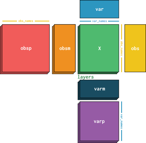
Note that all matrices in obsp must have shape (n_cells, n_cells) and use obs_names as an index to both dimensions. Similarly, varp must be (n_genes x n_genes) and use var_names to index.

Our example data now holds the following cell-cell pair matrix:

adata.obsp

PairwiseArrays with keys: distances_all

distances_all is the the full distance matrix between all pairs of cells.

As before with obsm and layers, obsp is a Python dictionary, so we can access the distance matrix by its key:

adata.obsp["distances_all"]

array([[ 0.        , 18.98223389, 15.39625646, ..., 17.44791227,
        19.66225537, 13.4530516 ],
       [18.98223389,  0.        , 21.37320952, ..., 17.39917931,
        16.59099551, 20.29010799],
       [15.39625646, 21.37320952,  0.        , ..., 17.48199881,
        19.54703132, 13.22466662],
       ...,
       [17.44791227, 17.39917931, 17.48199881, ...,  0.        ,
        14.53959947, 14.15720293],
       [19.66225537, 16.59099551, 19.54703132, ..., 14.53959947,
         0.        , 16.96518854],
       [13.4530516 , 20.29010799, 13.22466662, ..., 14.15720293,
        16.96518854,  0.        ]])

Lets have a closer look at the full distance matrix and plot it!

# plot distance matrix
plt.imshow(adata.obsp["distances_all"])
plt.colorbar(label="Euclidean distance in PCA space")
plt.show()

Here, we cannot see much structure. This is because the order of the cells is random! Therefore, let’s re-order the cells such that they are sorted by cell type before plotting:

# generate numerical index to sort cells by louvain cluster assignments
reorder_by_celltype = np.argsort(adata.obs["louvain_cell_types"])
# same distance matrix plot as before, but with `adata` reordered!
plt.imshow(adata[reorder_by_celltype, :].obsp["distances_all"])
plt.colorbar(label="Euclidean distance in PCA space")
plt.show()

Now, we can clearly see the block structure of the cell-cell distance matrix.

In summary, the obsp and varp fields allow to hold any kind of cell-cell or gene-gene paired data.

Unstructured annotations or general metadata in uns

Finally, there is only one subfield left! If we have metadata that does not fit any of the other fields or that describes the whole dataset and not specific cells or genes, we can store it as unstructured annotation in adata.uns:

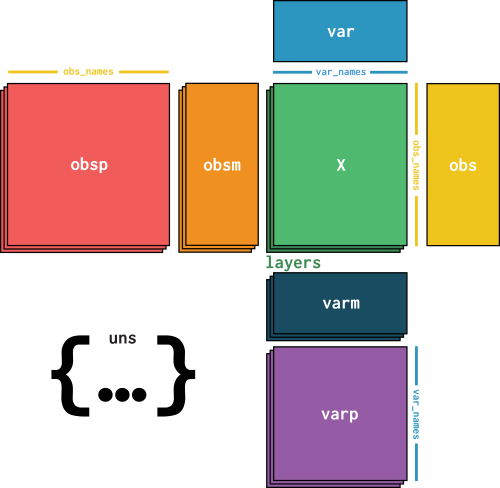
adata.uns is another Python dictionary, so we can access its contents via its keys:

adata.uns_keys()

['louvain', 'louvain_colors', 'pca']

In our example, uns holds some processing parameters or intermediate results of the methods that were already run on the data.

Let’s look at the pca and louvain fields:

# louvain clustering parameters
print(adata.uns["louvain"])

{'params': {'random_state': array([0]), 'resolution': array([1])}}

# louvain clustering plotting colors
print(adata.uns["louvain_colors"])

['#1f77b4' '#ff7f0e' '#2ca02c' '#d62728' '#9467bd' '#8c564b' '#e377c2'
 '#bcbd22']

# PCA: variance explained
print(adata.uns["pca"])

{'variance': array([32.11044  , 18.718647 , 15.607319 , 13.235274 ,  4.8012376,
        3.977329 ,  3.5053132,  3.1576602,  3.028463 ,  2.9777625,
        2.8842385,  2.8583548,  2.849085 ,  2.8220255,  2.811057 ,
        2.781576 ,  2.7436602,  2.7404478,  2.736062 ,  2.6872916,
        2.671316 ,  2.6690092,  2.6442325,  2.6394093,  2.6157827,
        2.6102393,  2.575101 ,  2.5691617,  2.563295 ,  2.5489197,
        2.5080354,  2.4762378,  2.264355 ,  2.1844513,  2.1353922,
        2.096509 ,  2.0606086,  2.0105643,  1.9703175,  1.9465197,
        1.9220033,  1.8847997,  1.8349565,  1.8038161,  1.7930729,
        1.7611799,  1.7322571,  1.721284 ,  1.6937429,  1.6519767],
      dtype=float32), 'variance_ratio': array([0.02012818, 0.01173364, 0.00978333, 0.00829643, 0.00300962,
       0.00249316, 0.00219728, 0.00197936, 0.00189837, 0.00186659,
       0.00180796, 0.00179174, 0.00178593, 0.00176896, 0.00176209,
       0.00174361, 0.00171984, 0.00171783, 0.00171508, 0.00168451,
       0.00167449, 0.00167305, 0.00165752, 0.00165449, 0.00163968,
       0.00163621, 0.00161418, 0.00161046, 0.00160678, 0.00159777,
       0.00157214, 0.00155221, 0.00141939, 0.00136931, 0.00133855,
       0.00131418, 0.00129168, 0.00126031, 0.00123508, 0.00122016,
       0.00120479, 0.00118147, 0.00115023, 0.00113071, 0.00112397,
       0.00110398, 0.00108585, 0.00107897, 0.00106171, 0.00103553],
      dtype=float32)}

In summary, the adata.uns field is helpful to store metadata that relates to the dataset as a whole (processing parameters, experimental details etc.).

Views and copies of AnnData objects

As we mentioned in the section on subsetting, whenever you subset an AnnData objects, you will always get a view in return instead of making a copy. That avoids having the same data in memory twice. Sometimes you will want to have a copy instead of a view, i.e. to modify the subset independent of the parent AnnData object. We will get to that below - but first, let’s demonstrate what a “view” is.

For that, we first look at a 5x5 subset of our active data matrix, by indexing X directly. We add .A to turn the sparse X into a nice print-out:

adata.X[:5, 5:10].A

array([[0.        , 0.        , 0.        , 0.        , 0.        ],
       [0.        , 0.        , 0.        , 0.64266497, 0.        ],
       [0.532456  , 0.        , 0.        , 0.        , 0.        ],
       [2.1446393 , 0.        , 0.        , 0.        , 0.        ],
       [0.        , 0.        , 0.        , 0.        , 0.        ]],
      dtype=float32)

Now, if we index adata directly, we get a “view” - that means it does not copy the data of our 5x5 subset and stores it somewhere. Instead, when we use it, it will use the data of the original AnnData object that is already in memory.

adata_view = adata[:5, 5:10]
adata_view

View of AnnData object with n_obs × n_vars = 5 × 5
    obs: 'n_genes', 'percent_mito', 'n_counts', 'louvain_cell_types', 'is_low_quality'
    var: 'gene_names', 'n_cells', 'gene_ids'
    uns: 'louvain', 'louvain_colors', 'pca'
    obsm: 'X_pca', 'X_tsne', 'X_umap'
    layers: 'raw', 'counts_per_million'
    obsp: 'distances_all'

Of course, the data inside the .X of our adata_view is exactly our subset from above:

adata_view.X.A

array([[0.        , 0.        , 0.        , 0.        , 0.        ],
       [0.        , 0.        , 0.        , 0.64266497, 0.        ],
       [0.532456  , 0.        , 0.        , 0.        , 0.        ],
       [2.1446393 , 0.        , 0.        , 0.        , 0.        ],
       [0.        , 0.        , 0.        , 0.        , 0.        ]],
      dtype=float32)

However, what if we change something in the parent AnnData object? Lets add a fake value in the first row of the original adata.X and then check what happens see what happens in the X of the view:

adata.X[0, 7] = 99
adata_view.X.A

array([[ 0.        ,  0.        , 99.        ,  0.        ,  0.        ],
       [ 0.        ,  0.        ,  0.        ,  0.64266497,  0.        ],
       [ 0.532456  ,  0.        ,  0.        ,  0.        ,  0.        ],
       [ 2.1446393 ,  0.        ,  0.        ,  0.        ,  0.        ],
       [ 0.        ,  0.        ,  0.        ,  0.        ,  0.        ]],
      dtype=float32)

The change propagated as expected! Because the view just mirrors the parent AnnData object, we can see the fake value inserted in the parent X also in the view.

Note

Propagating changes from a parent AnnData object to its view(s) currently works for all numpy-derived fields (X, layers, obsm, varm, obsp and varp) but not for the pandas-derived obs and var dataframes! See this github issue for status updates.

Turn a view into a copy

As mentioned above, sometimes you might want a copy of the parent AnnData instead of just a view. You can get an actual AnnData object from a view in two ways:

• call .copy() on the view - a copy is returned

• modify any of elements of the view - the view object will be turned into copy

Lets try this - we start with the adata_view that we created above:

adata_view  # still a view

View of AnnData object with n_obs × n_vars = 5 × 5
    obs: 'n_genes', 'percent_mito', 'n_counts', 'louvain_cell_types', 'is_low_quality'
    var: 'gene_names', 'n_cells', 'gene_ids'
    uns: 'louvain', 'louvain_colors', 'pca'
    obsm: 'X_pca', 'X_tsne', 'X_umap'
    layers: 'raw', 'counts_per_million'
    obsp: 'distances_all'

adata_view_copy = adata_view.copy()
adata_view_copy  # an actual AnnData object!

AnnData object with n_obs × n_vars = 5 × 5
    obs: 'n_genes', 'percent_mito', 'n_counts', 'louvain_cell_types', 'is_low_quality'
    var: 'gene_names', 'n_cells', 'gene_ids'
    uns: 'louvain', 'louvain_colors', 'pca'
    obsm: 'X_pca', 'X_tsne', 'X_umap'
    layers: 'raw', 'counts_per_million'
    obsp: 'distances_all'

adata_view.obs["new_column"] = "Test"  # add a new column to the `obs` dataframe
adata_view  # Not a view anymore!

AnnData object with n_obs × n_vars = 5 × 5
    obs: 'n_genes', 'percent_mito', 'n_counts', 'louvain_cell_types', 'is_low_quality', 'new_column'
    var: 'gene_names', 'n_cells', 'gene_ids'
    uns: 'louvain', 'louvain_colors', 'pca'
    obsm: 'X_pca', 'X_tsne', 'X_umap'
    layers: 'raw', 'counts_per_million'
    obsp: 'distances_all'

Note that when we modified the adata_view, this not only turned adata_view into a propper AnnData object by making a copy internally - it also triggered the ImplicitModificationWarning to let you know what happened.

Now, both adata_view_copy and adata_view store actual data and are separated from their parent AnnData object adata. We can demonstrate that by adding another fake value to adata.X as before:

adata.X[0, 8] = 98
adata.X[:5, 5:10].A  # the parent of course has the change

array([[ 0.        ,  0.        , 99.        , 98.        ,  0.        ],
       [ 0.        ,  0.        ,  0.        ,  0.64266497,  0.        ],
       [ 0.532456  ,  0.        ,  0.        ,  0.        ,  0.        ],
       [ 2.1446393 ,  0.        ,  0.        ,  0.        ,  0.        ],
       [ 0.        ,  0.        ,  0.        ,  0.        ,  0.        ]],
      dtype=float32)

adata_view.X.A  # the former view (that now is a actual AnnData object) does not have it

array([[ 0.        ,  0.        , 99.        ,  0.        ,  0.        ],
       [ 0.        ,  0.        ,  0.        ,  0.64266497,  0.        ],
       [ 0.532456  ,  0.        ,  0.        ,  0.        ,  0.        ],
       [ 2.1446393 ,  0.        ,  0.        ,  0.        ,  0.        ],
       [ 0.        ,  0.        ,  0.        ,  0.        ,  0.        ]],
      dtype=float32)

adata_view_copy.X.A  # the copy of the view (also an actual AnnData object) does not have it either

array([[ 0.        ,  0.        , 99.        ,  0.        ,  0.        ],
       [ 0.        ,  0.        ,  0.        ,  0.64266497,  0.        ],
       [ 0.532456  ,  0.        ,  0.        ,  0.        ,  0.        ],
       [ 2.1446393 ,  0.        ,  0.        ,  0.        ,  0.        ],
       [ 0.        ,  0.        ,  0.        ,  0.        ,  0.        ]],
      dtype=float32)

In summary, views can help to quickly create a subset of an existing AnnData object without using additional memory. However, if you modify them, they will turn into an actual AnnData object and contain a separate copy of the data you subsetted.

Where can I get help, and what tutorial should I try next?

This is the end of the this introductory tutorial. You can find more details on anndata functionality on the documentation page. On the anndata [GitHub] you can read about and report new technical issues. On the scverse Discord you can ask questions to the scverse community and get help from our developers.

MuData: AnnData, but for multimodal datasets

mudata is the extension of anndata to multimodal datasets, i.e. whenever you have high-dimensional observations from more than one modality (e.g. combined scRNA and scATAC data) and want to manage annotations of cells/genes/… in a consistent and convenient way. It builds intuitively on anndata by treating the data from each modality as a separate AnnData object, but combining them to a joint, multimodal way in the MuData object. Try the introductory tutorial to get started, and see the page on multimodal data containers to get a first overview of the MuData object and its contents.

Advanced tutorials

For some advanced topics, we have dedicated tutorials that you can try next. They can be found on the scverse tutorial page. Here are a few recommendations:

• Coming to Python&scverse from R? Try our interoperability tutorial, where we show how AnnData objects can be interfaced with single cell data structures from other languages (e.g. Seurat. SingleCellExperiment, …)

• Work with large datasets and don’t want to fully load them into memory? Check out our anndatas backed mode tutorial

• Want to combine datasets? We a tutorial on how axes and concatenation work for both AnnData and MuData objects.